p-value distribution

Primer

In null-hypothesis significance testing, p-value is the probability of obtaining test results at least as extreme as the result actually observed, under the assumption that the null hypothesis is correct. Another way to put it, p-values tell you how surprising the data is, assuming there is no effect.

Type-I & Type-II Errors

• Type-I Error (false positive): mistakenly reject null hypothesis when null hypothesis is actually true.
• Type-II Error (false negative): failure to reject null hypothesis when alternative hypothesis is true.

Significance Level & Statistical Power

• Significance Level (alpha): $\alpha$ = probability of Type I error.
• Statistical Power (beta): the probability of observing a significant effect if there is a true effect. $\beta$ = 1 - probability of Type_II_Error.

Statistical Significance

If the p-value is less than the significance level, the result is considered statistically significant and the null hypothesis is rejected. If the p-value is greater than the significance level, the result is not statistically significant and the null hypothesis is not rejected.

Problem Statement

Which p-values can you expect to observe if there is no effect vs. if there is a true effect?

We simply know that:

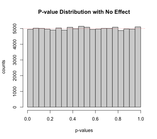
1. If there is no effect, p-value is likely to be greater than the significance level $\alpha$, but there is still some chance that p-value is less than the significance level, leading to Type I error. By definition, that chance equals to $\alpha$.

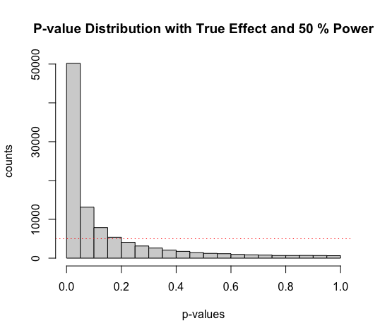
2. If there is a true effect, p-value is likely to be less than the significance level $\alpha$, and its probability depends on the statistical power.

We seek more insights through simulations below.

Simulation

library(pwr)

n_sims <- 100000  # number of simulated experiments

population_mean <- 100

# parameters that can be changed in simulations
sample_mean <- 106
sample_size <- 26
sample_sd <- 15
alpha <- 0.05

# run simulations
p_values <- numeric(n_sims)
for (i in 1:n_sims) {
    samples <- rnorm(n=sample_size, mean=sample_mean, sd=sample_sd)
    t_test <- t.test(samples, mu=population_mean, alternative='two.sided')
    p_values[i] <- t_test$p.value
}
cat("simulated power (probability of significat effect i.e. p-value < alpha, assuming a true effect):\n", sum(p_values < alpha)/n_sims)

# calculate power formally by power analysis
power_calc <- pwr.t.test(n=sample_size, d=(sample_mean - population_mean)/sample_sd, sig.level=alpha, type='one.sample', alternative='two.sided')
power <- power_calc$power

# plot
n_bars <- 20
hist(p_values, main=paste("P-value Distribution with True Effect and", round(power*100, digit=1), "% Power"), xlab="p-values", ylab="counts", breaks=n_bars)
# the red dotted line indicates the frequency in each bar, assuming the null hypothesis is true
abline(h=n_sims/n_bars, col="red", lty=3)

• the code represents a true effect and power of 50%

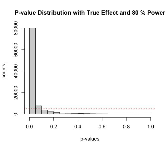
• increasing sample_size from 26 to 51 will increase the power from 50% to 80%

sample_size <- 51

• setting sample_mean equals to population_mean denotes a design of no true effect

sample_mean <- 100
...
n_bars <- 100
hist(p_values, main="P-value Distribution with No Effect", xlab="p-values", ylab="counts", breaks=n_bars)
...

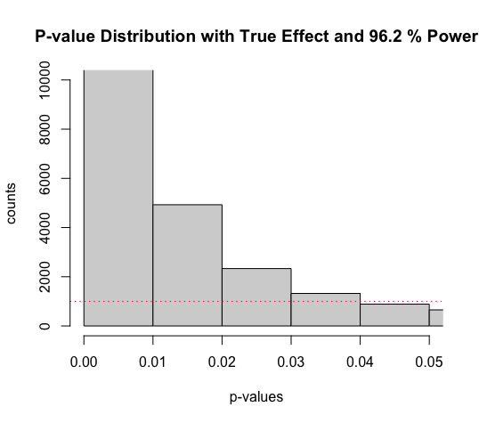
• increasing sample_size from 26 to 51 and increasing sample_mean from 106 to 108 will increase the power further to 96%.

sample_mean <- 108
sample_size <- 51
...
n_bars <- 100
hist(p_values, main=paste("P-value Distribution with True Effect and", round(power*100, digit=1), "% Power"), xlab="p-values", ylab="counts", xlim=c(0, 0.05), ylim=c(0, 10000), breaks=n_bars)
...

We see in the figure above that the bar with p-values between 0.04 and 0.05 is lower than the red line (frequency in each bar assuming the null hypothesis is true). When the null hypothesis is true, p-values between 0.04 and 0.05 occur exactly 1% of the time (because p-values are uniformly distributed); when there is true effect and power is very high, p-values between 0.04 and 0.05 are very rare – they occur less than 1% of the time.

Supposing you have very high power, use an alpha level of 0.05, and find a p-value of p = 0.045, the data is surprising assuming the null hypothesis is true, but it is even more surprising, assuming the alternative hypothesis is true. This shows how a significant p-value is not always evidence for the alternative hypothesis.

Lindley’s paradox: a result can be unlikely when the null hypothesis is true, but it can be even more unlikely assuming the alternative hypothesis is true, and power is very high.

Conclusion

• When there is no true effect, p-values are uniformly distributed.

• When there is a true effect, p-value distribution depends on the statistical power: the higher the power, the more p-values fall below 0.05, and the steeper the p-value distribution becomes.

Reference

Daniel Lakens, Which p-values can you expect, Improving your statistical inferences, 2016, Coursera.